
You don’t have to manually format your data with colors and styles to make it stand out. With conditional formatting in Microsoft Excel, you can automatically format your dataset based on conditions. Plus, Excel gives you five preset conditional formatting options to make this task an easy one.
Note: keep in mind with all the conditional formatting rules below that if you change the cell data, and it no longer meets the criteria, the formatting will be removed.
Highlight Cell Rules
Using rules to highlight cells based on a value, text, or date is probably the most popular type of conditional formatting in Excel. With this option, you can do things like highlight cells with values that are greater than or less than another, text that contains something in particular, a date occurring in a certain time frame, or duplicate values.
Highlight Values
If you’re using values like numbers, currencies, or percentages in your sheet, you can highlight values as they relate to others. You could format sales greater than or inventory less than a given amount.
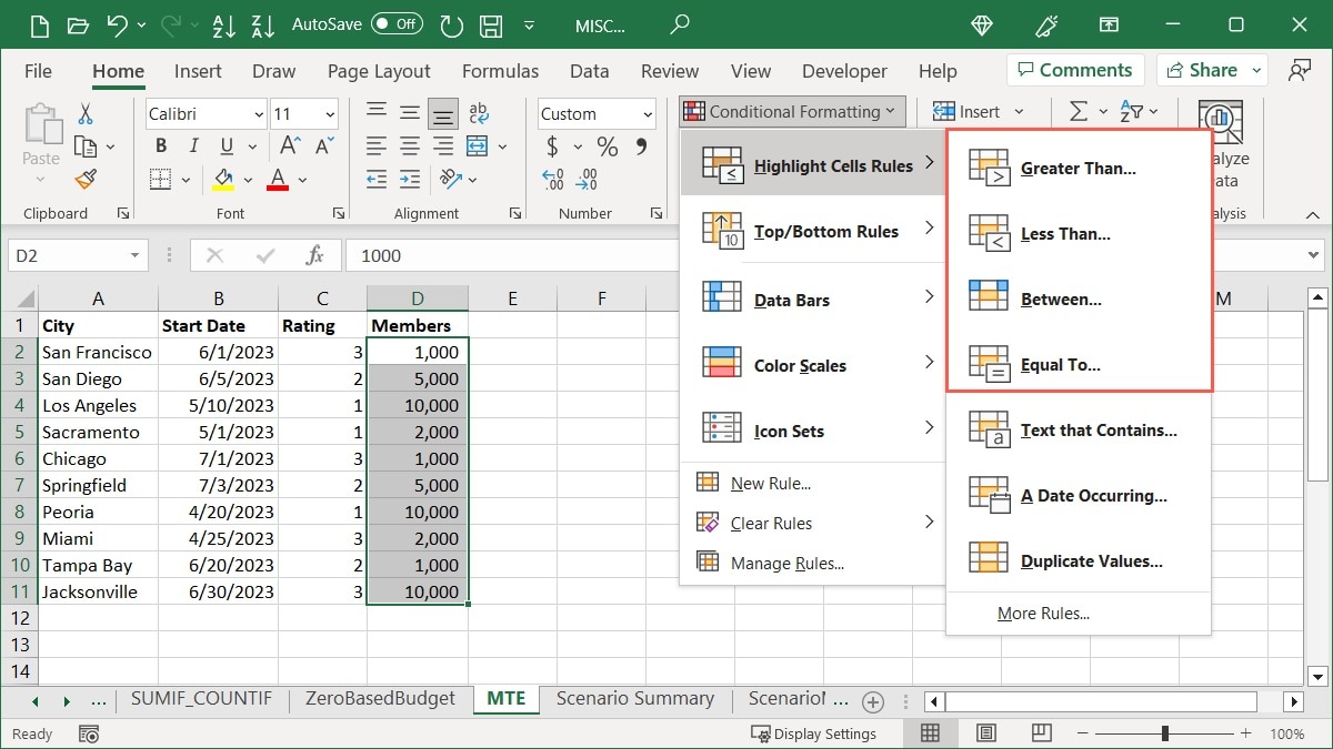
- Select the cells you want to test, go to the “Home” tab, open the “Conditional Formatting” drop-down menu, select “Highlight Cell Rules,” then choose the condition you would like to use.
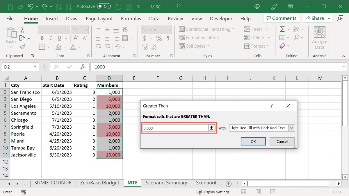
- Enter the comparison value in the field on the left of the pop-up box. Alternatively, enter a cell reference containing that value. For instance, we’re highlighting cells in our selected range that are greater than “3,000.”
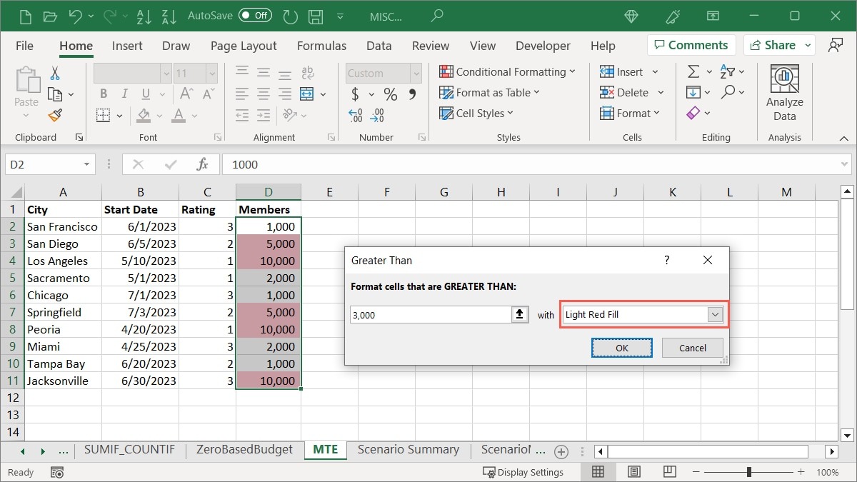
- Choose the highlighting to apply in the drop-down list to the right. We’re choosing “Light Red Fill.”
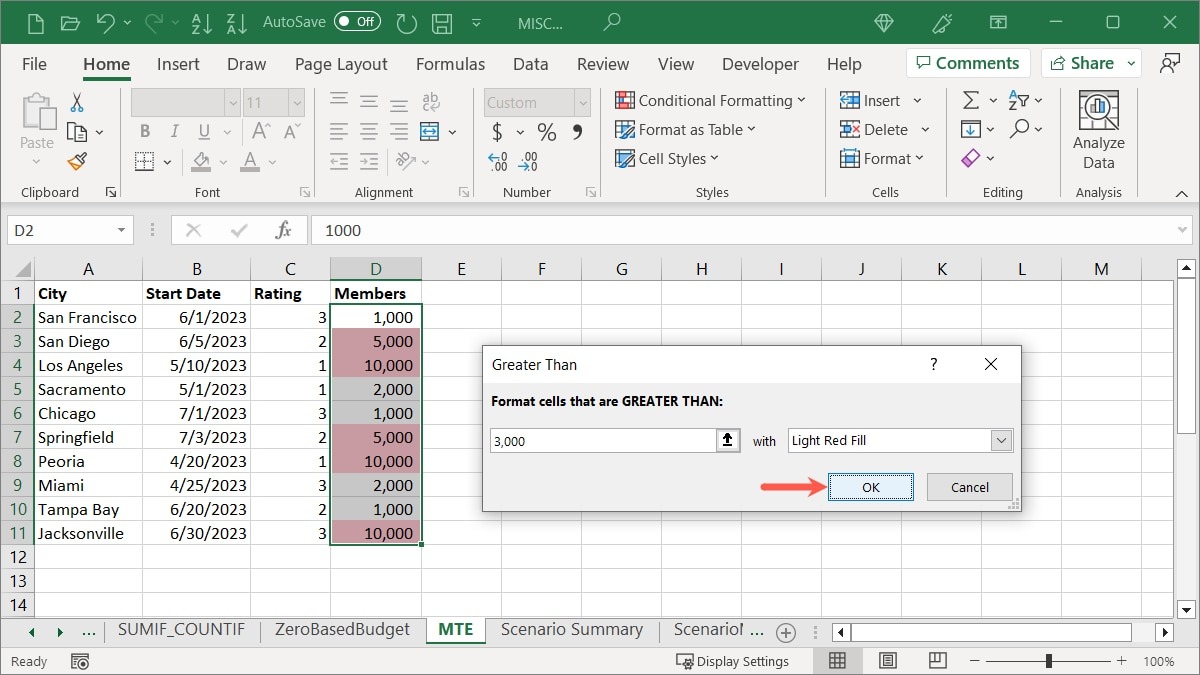
- Click “OK” to apply and save the formatting.
Highlight Text
Perhaps it’s particular text in your cells that you want to highlight. You can use a word or even a single letter for your condition. You could format names of employees, cities or states, or letter grades.
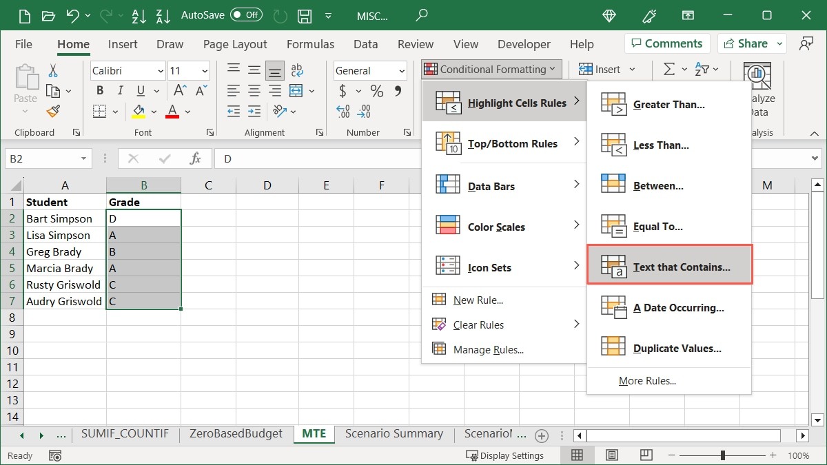
- Select the cells you want to check, go to the “Home” tab, open the “Conditional Formatting” drop-down menu, select “Highlight Cell Rules,” and choose “Text That Contains.”
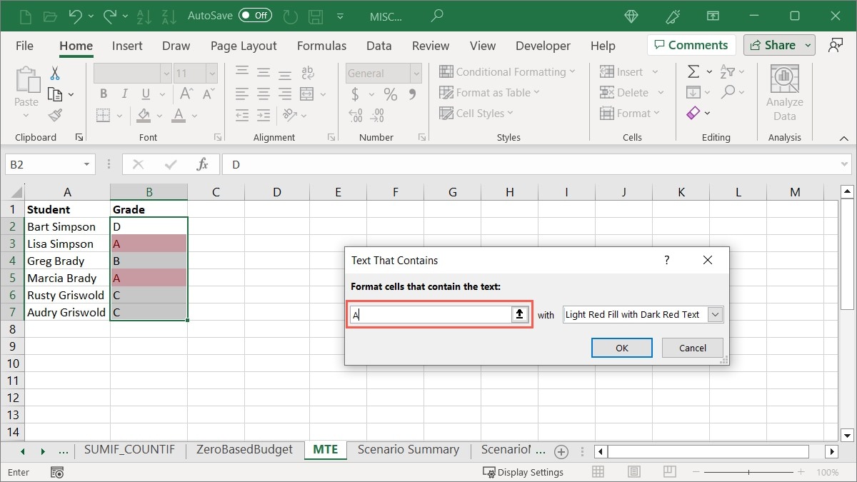
- Enter the text in the field on the left of the pop-up box. For example, we’re highlighting cells that contain the letter grade “A.”
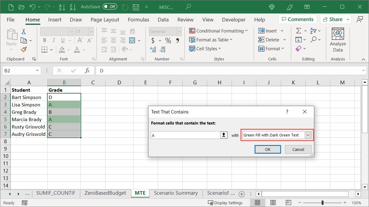
- Choose the highlighting in the list on the right. We’re choosing “Green Fill with Dark Green Text.”
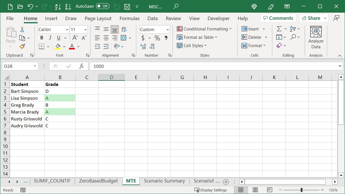
- Click “OK” to apply your formatting.
Highlight Dates
Another way to highlight values is using dates. You could choose a specific color for due dates for upcoming bills or tasks with dates from the past.
- Select the cells you want to check, go to the “Home” tab, open the “Conditional Formatting” drop-down menu, select “Highlight Cell Rules,” and choose “A Date Occurring.”
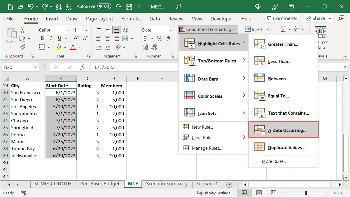
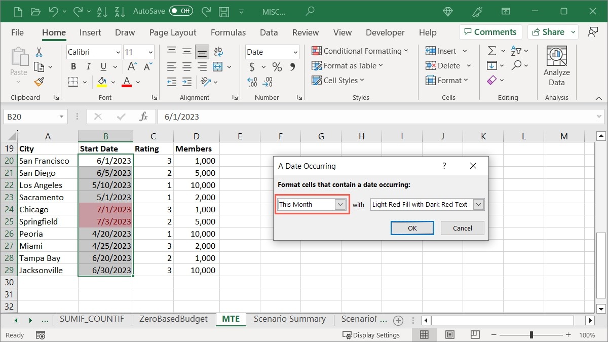
- Choose a time frame in the pop-up box. As an example, we’re choosing “This Month.”
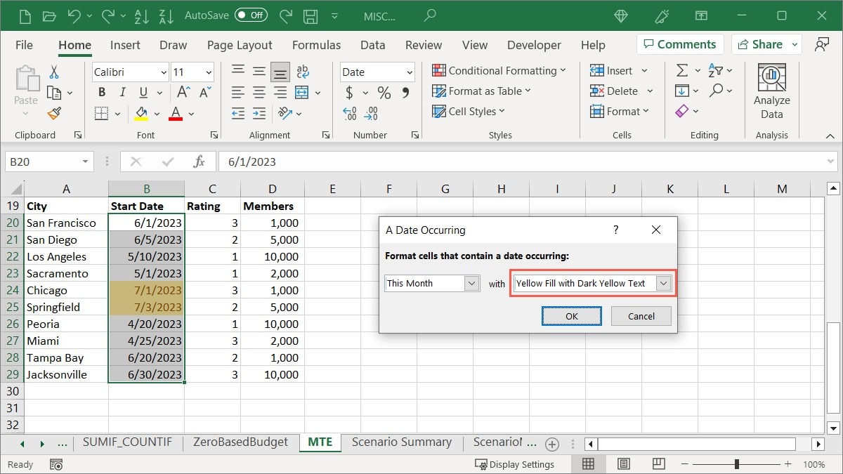
- Choose the highlighting from the list on the right. We’re selecting “Yellow Fill with Dark Yellow Text.”
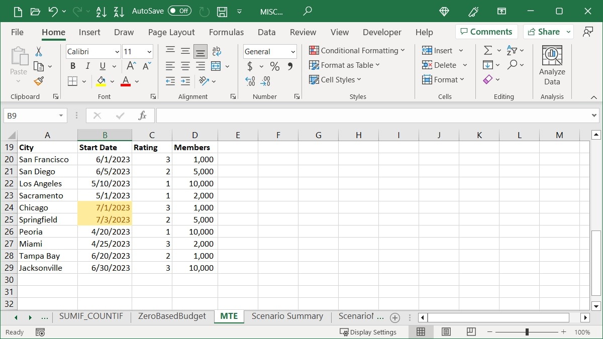
- Click “OK” to save the formatting.
Tip: if you’re interested in highlighting duplicate values in your sheet using that conditional formatting option, check out our complete how-to for finding and removing duplicates in Excel.
Apply Top or Bottom Rules
If you want to highlight things like top sales, bottom test scores, or above average quarterly profits, you can use the Top or Bottom Rules conditional formatting option.
Highlight a Top Percentage
Perhaps you’re looking for the top numbers from a group of cells. You can highlight a top percentage and adjust that percentage if you would like.
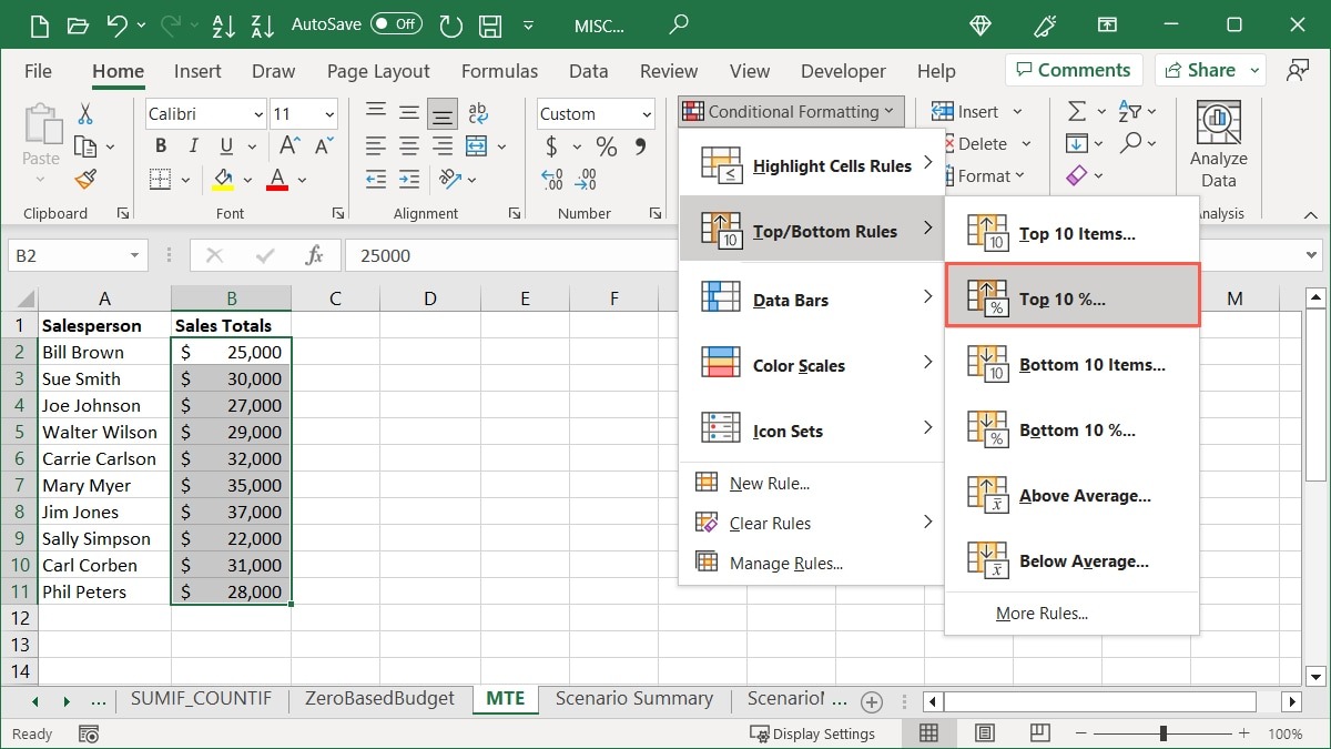
- Select the cells you want to test, go to the “Home” tab, open the “Conditional Formatting” drop-down menu, move to “Top/Bottom Rules,” and choose “Top 10%.”
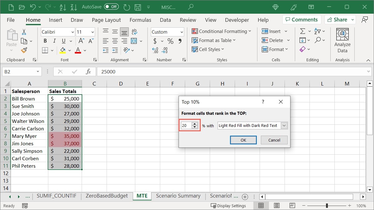
- Leave the number “10” in the field on the left of the pop-up box, or adjust that percentage by entering a number or using the arrows. For example, we’re changing it to view the top “20” percent.
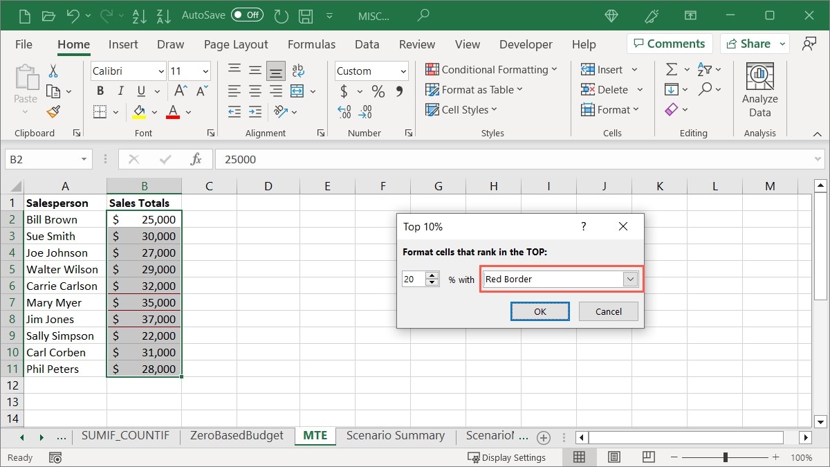
- Choose the formatting you want to apply in the list on the right. We are choosing “Red Border.”
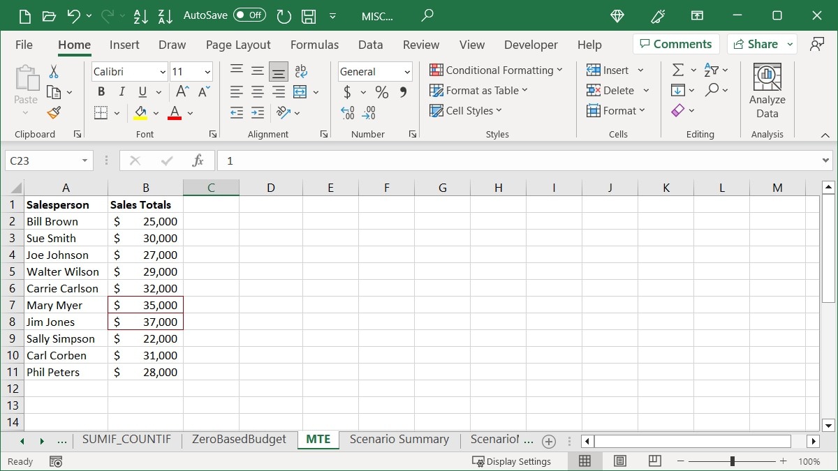
- Click “OK” to save and apply the formatting after seeing a preview.
Highlight Below Average
You can also highlight the amounts below average.
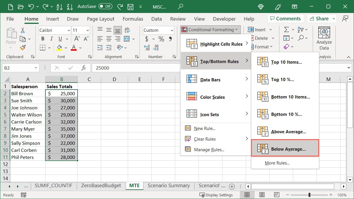
- Select the cells, go to the “Home” tab, open the “Conditional Formatting” drop-down menu, move to “Top/Bottom Rules,” and choose “Below Average.”
- Choose the formatting you want to apply, then click “OK.” We’re choosing “Custom Format,” then selecting “Bold Italic” in the next window.
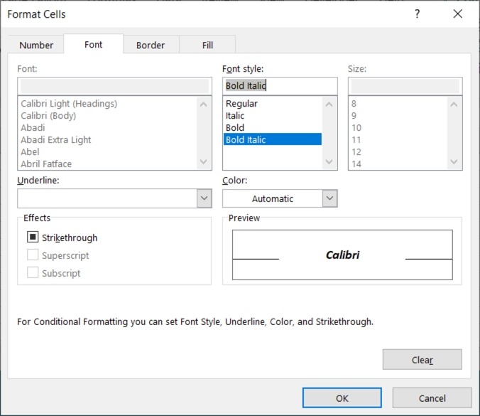
- Select “OK” to save the formatting you see in the preview.

Tip: did you know that you can also use conditional formatting in Microsoft Outlook to make certain emails pop? Take a look at our how-to for setting this up.
Use Data Bars
Another useful conditional formatting in Excel is Data Bars. You can apply colored bars to your cells, where the length of each bar represents the cell’s value. This offers a quick view of high and low numbers, like a city’s population, product inventory, or revenue by location.
- Select the cells you want to format, go to the “Home” tab, open the “Conditional Formatting” drop-down menu, and select “Data Bars” to see gradient and solid fill options.
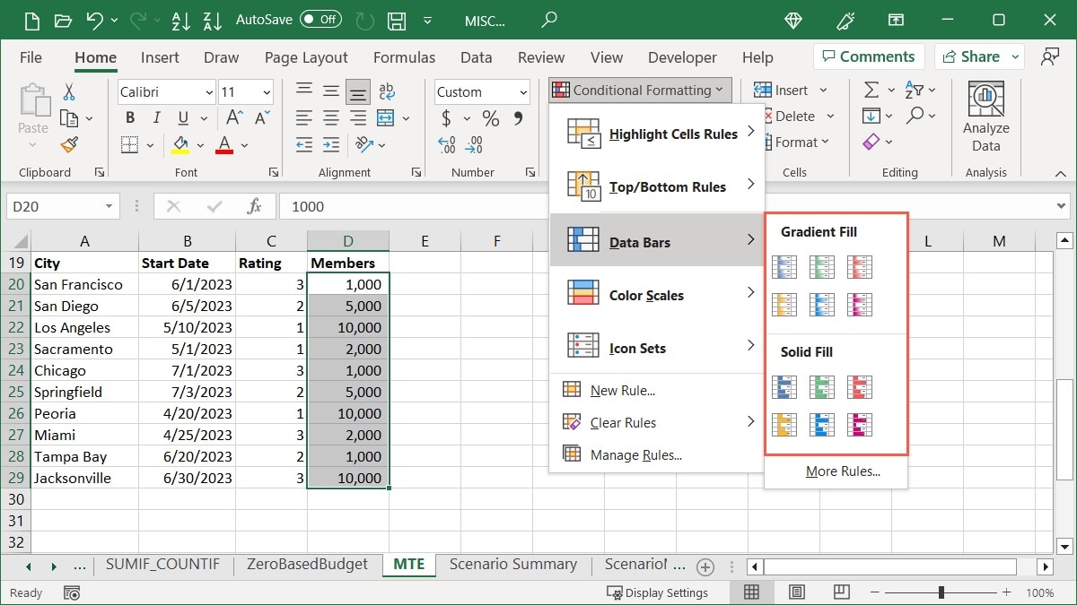
- As you hover your cursor over each Data Bar option, you’ll see a preview in your selected cells.
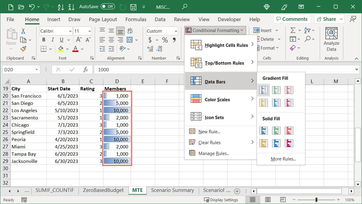
- Click the style and color you want to use.
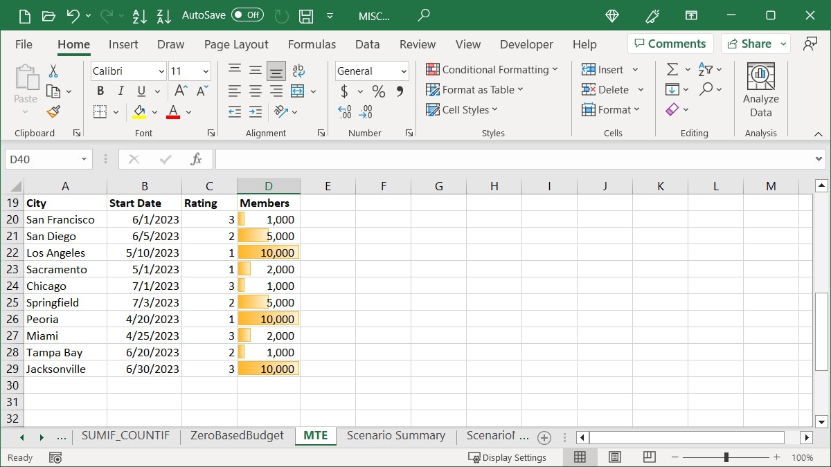
Note: instead of data bars, you could use Excel’s sparklines to spot a trend in your data. Sparklines are single cell mini charts that visualize a set range of data.
Add Color Scales
Maybe you like the splash of color for quickly identifying values, but prefer different colors to represent the values. With Color Scales, the colors change according to how high or low the values are.
This type of formatting is used with heat maps showing temperatures, populations, or income by region, but you can use it just as easily for sales, revenue, or expenses.
- Select the cells you want to format, go to the “Home” tab, open the “Conditional Formatting” drop-down menu, and select “Color Scales” to see the color options.
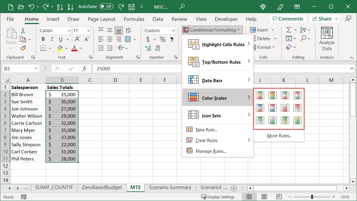
- Hover your cursor over each Color Scale to see a preview, then make your selection. You can use a two- or three-color scale, depending on the number of items you’re comparing.
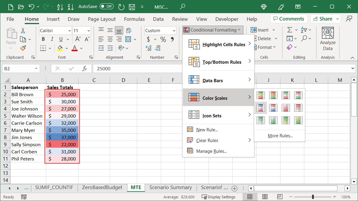
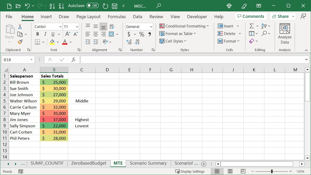
The first color in the scale represents the highest value in the group. Large groups of items will show different shades of the colors as the differences between the values. As an example, we’re selecting the “Red Yellow Green” option.
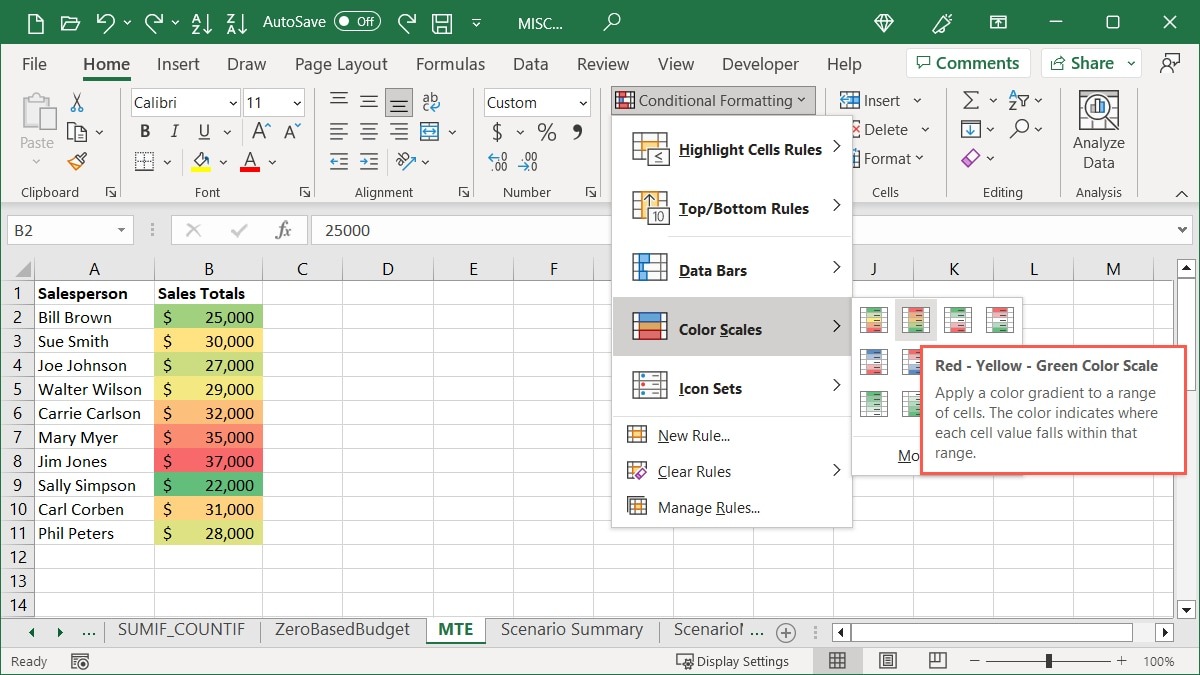
The highest values are in red, the middle values in yellow, and the lowest values in green, with the values in between in different shades of those colors.
Tip: if you’re struggling to get the right results because your spreadsheet is a mess, try cleaning up your data first.
Insert Icon Sets
Another conditional formatting option you’ll see in Excel is the Icon Sets. This type of formatting places icons next to the cells in your group, based on their values.
The collection of icons you use is up to you, but Excel offers some assistance by categorizing them as Directional, Shapes, Indicators, and Ratings. Additionally, you’ll notice that some sets contain different numbers of icons, which is also useful in selecting a set.
Select the cells you want to use, go to the “Home” tab, open the “Conditional Formatting” drop-down menu, select “Icon Sets,” then select the icon set you would like.
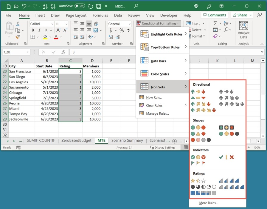
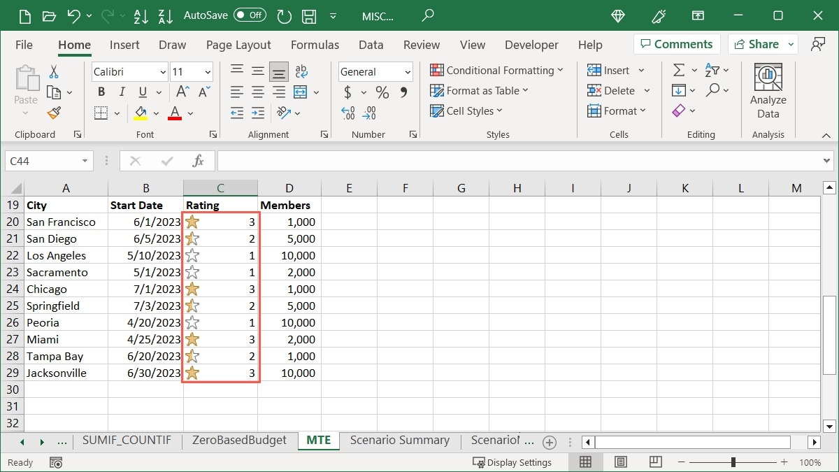
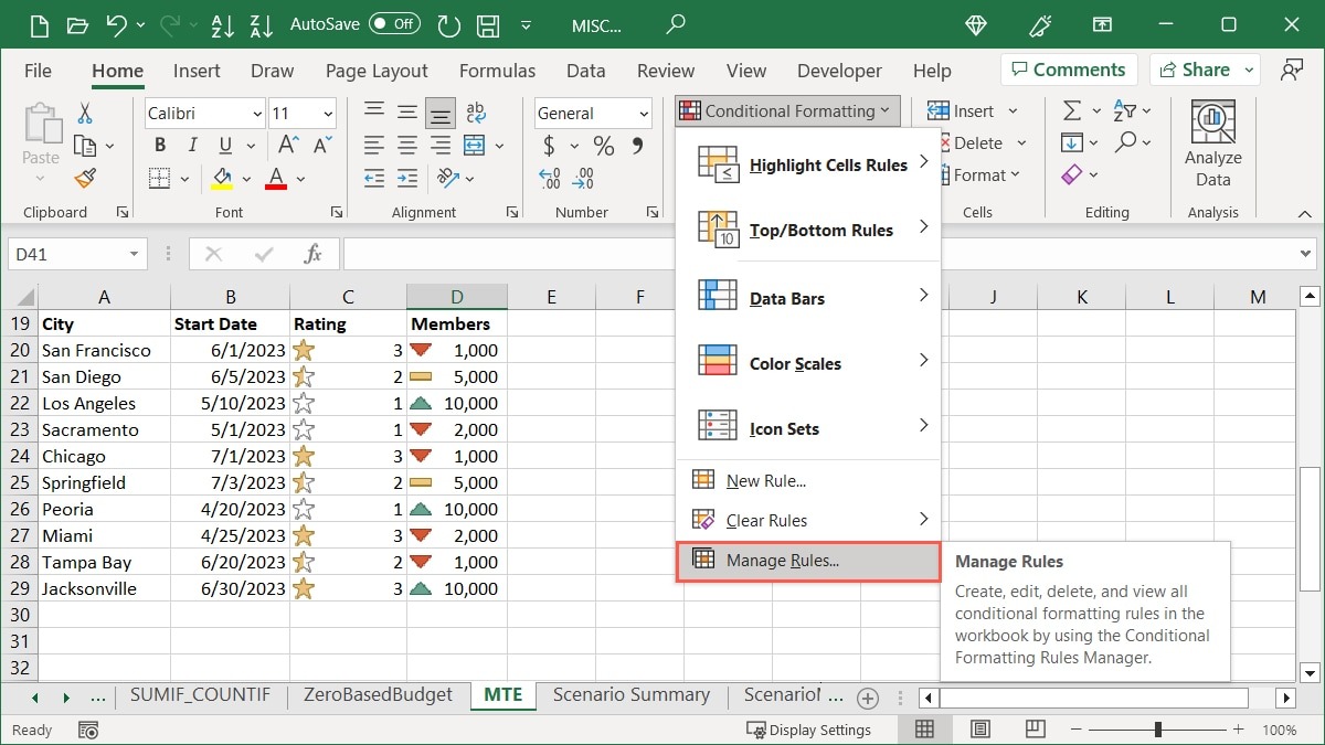
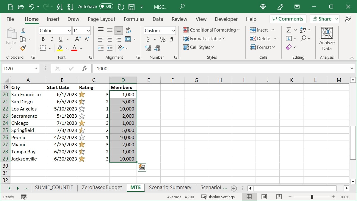
As an example, we have a range of ratings for our cities, so we’re selecting one of the “Ratings” sets. Since our ratings are on a scale of one to three, the “3 Stars” set is ideal.
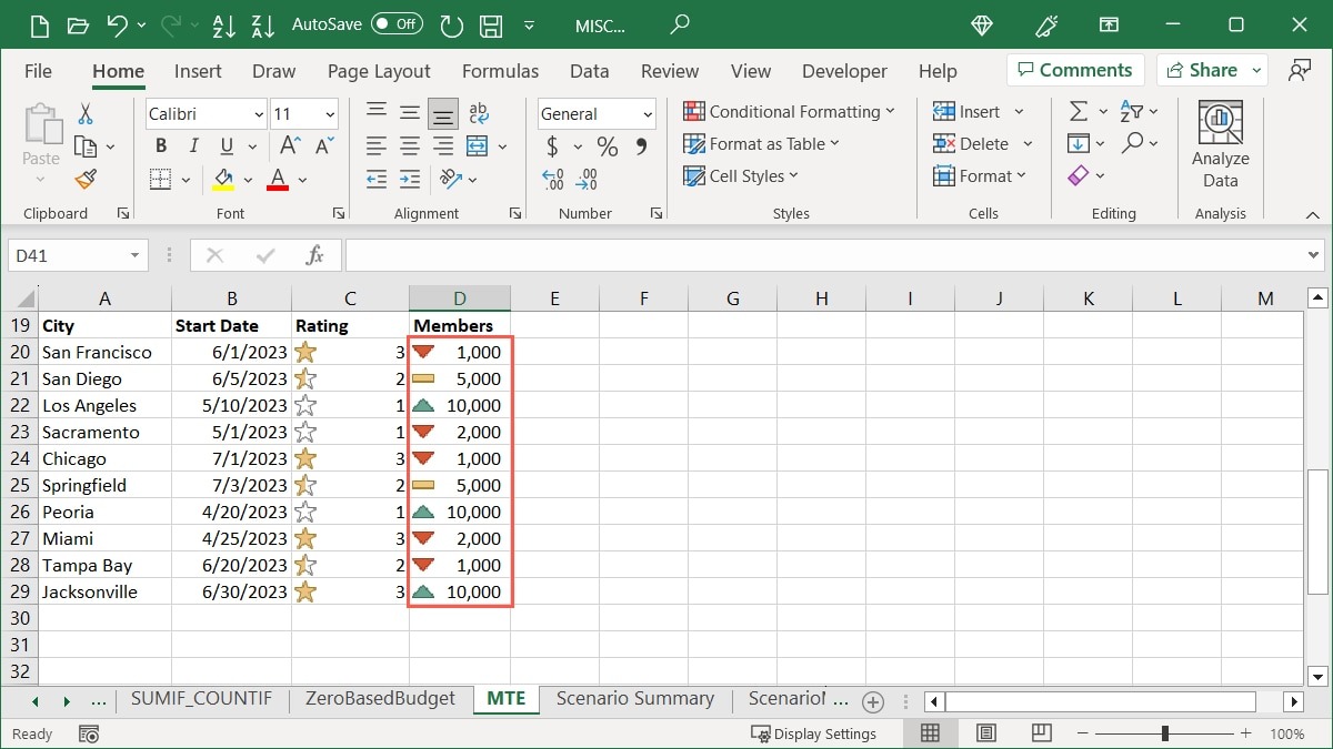
In another example, we have the number of members in each of our cities and want to quickly spot the highest and lowest. We’re choosing the “Directional” set and the “3 Triangles” option to see the highest numbers with a green up-pointing arrow, the middle numbers with a yellow rectangle, and the lowest numbers with a red down-pointing arrow.
How to Edit a Conditional Formatting Rule
Once you apply conditional formatting to your Excel sheet, you may want to make a change. Whether you’re making a change to the cell range or the formatting itself, you can edit an existing rule easily.
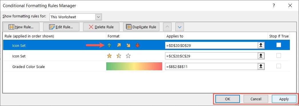
- Go to the “Home” tab, open the “Conditional Formatting” menu, and select “Manage Rules.”
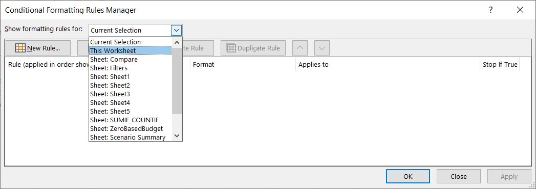
- Use the drop-down box at the top to choose the rules you want to see. You can view them for selected cells, the current worksheet, or a specific sheet in the workbook.
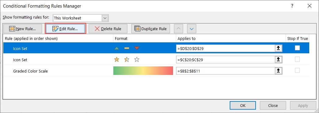
- If you only want to adjust the cell range, do so in the corresponding field below “Applies to.” Otherwise, click “Edit Rule” at the top.
- Make your changes in the “Edit Formatting Rule” box that opens, then click “OK,” In our example, we’re changing the Icon Style.
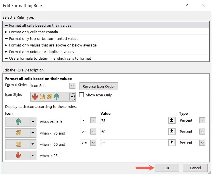
- Click “OK,” then “Apply” to save your changes.
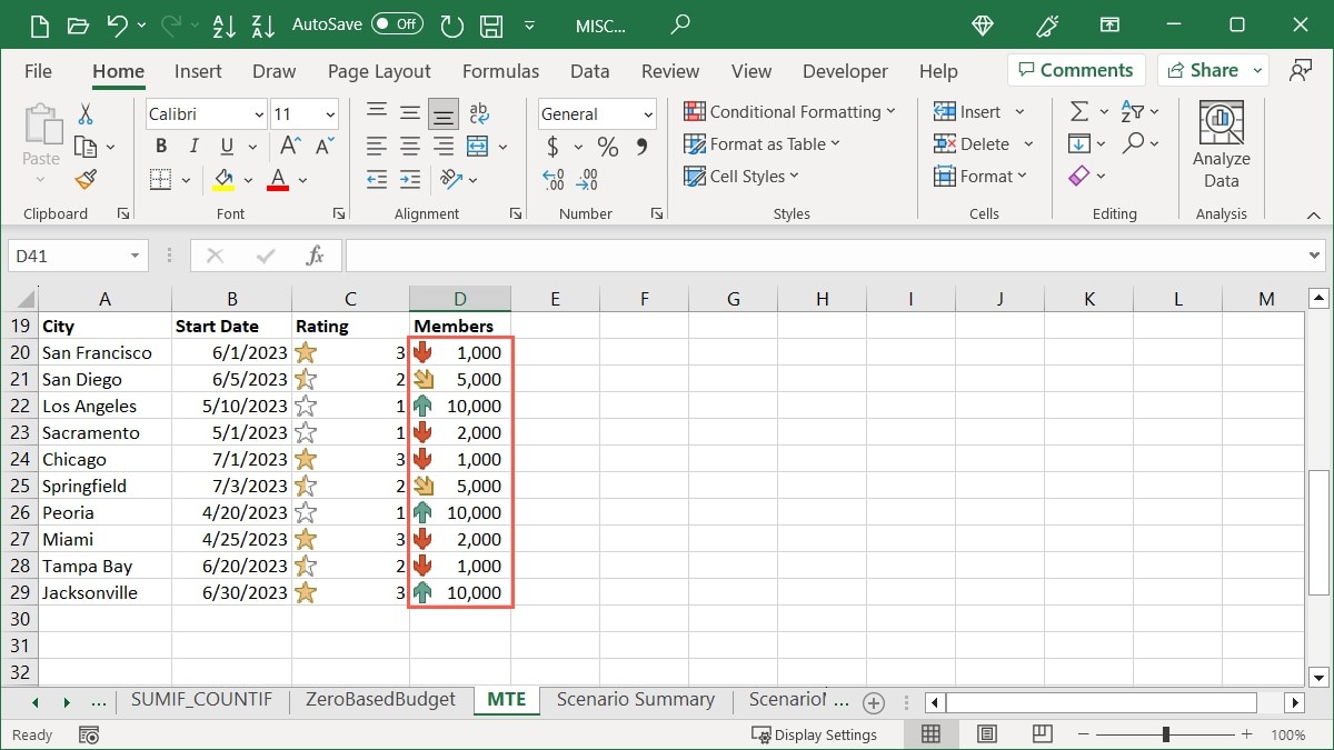
- Your sheet will update with your edits.
How to Delete a Conditional Formatting Rule
Should you decide you no longer want a conditional formatting rule you’ve set up, you can delete it one of two ways.
Use the Conditional Formatting Rules Manager
You can remove a rule in the Conditional Formatting Rules Manager with the click of a button.
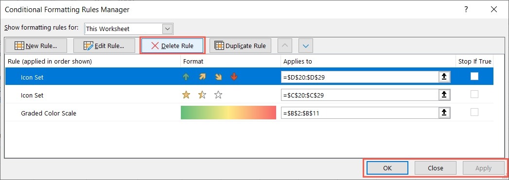
- Go to the “Home” tab, open the “Conditional Formatting” menu, and select “Manage Rules.”
- Select the rule, select “Delete Rule” at the top, then click “OK” and “Apply.”
Use the Clear Rules Option
Another way to remove a conditional formatting rule is using the Clear Rules option.
- Go to the “Home” tab, open the “Conditional Formatting” drop-down menu, move to “Clear Rules,” and choose to clear the rules from selected cells, the entire sheet, a table, or a pivot table. Note that if you don’t have a rule set up for a particular action, it’ll be grayed out.
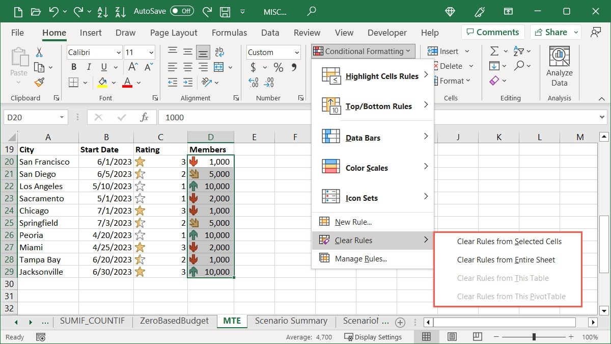
- Your rule will be removed.
Frequently Asked Questions
Can I have two conditional formatting rules for the same cells?
You can apply various conditional formatting rules to the same set of cells if you would like. For instance, you may want to highlight dates for last month in red text and dates for next month in green text. Follow the same steps you see here to add more rules to your selected cells, but be careful to not make your rules conflict with each other.
If it’s possible that all rules can apply, but it could cause a formatting problem, select the first rule for the cell range in the Conditional Formatting Rules Manager, then check the box for “Stop If True.” This stops the remaining rules from running, should they also apply.
Can I create my own conditional formatting rule?
Along with the preset conditional formatting rules shown here, you can set up your own. Select the cells you want to use, go to the “Home” tab, and click “Conditional Formatting -> New Rule.” Choose a rule type at the top, set up the rest of the rule in the section at the bottom, then click “OK” to save it.
Can I use conditional formatting to highlight an entire row or column?
You can set up a conditional formatting rule beyond a particular range of cells. So, yes, you can highlight an entire row or column based on conditions. Select the row or column, then set up your rule as described above. Keep in mind that if you have empty cells, you may not see formatting based on value, text, or date.
Image credit: Pixabay. All screenshots by Sandy Writtenhouse.
Our latest tutorials delivered straight to your inbox