
When you analyze your data in Microsoft Excel, you may want to do some comparisons, such as “What if I choose Option A instead of Option B?” Using the built-in What-If Analysis tools in Excel, you can compare numbers and amounts more easily – for example, to evaluate job salaries, loan options, or revenue and expense scenarios.
The What-If Analysis tools in Excel include the Scenario Manager, Goal Seek, and Data Table. To best explain the purpose of these tools, let’s look at examples of each.
Tip: lean how to remove duplicate and clean up data on Microsoft Excel.
Scenario Manager
Using the Scenario Manager, enter values that you can change to see varying results. As a bonus, create a Scenario Summary Report to compare the amounts or numbers side by side.
For example, say you’re planning an event and deciding between a few themes that have different costs. Set up each theme’s prices to see how much they’ll cost to compare them.
Create various scenarios for different situations to help in your decision-making.
How to Use the Scenario Manager
If you’re ready to compare different situations, like the example above, follow these steps to use the Scenario Manager in Excel.
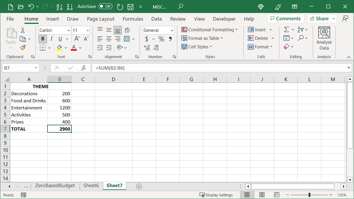
- Enter the data for your first scenario in your sheet. Using the earlier example, we are comparing theme costs for our event and entering the expenses for our Beach Theme in cells A2 through A6 and their costs in cells B2 through B6. We are adding the prices together in cell B7 to see the total cost.
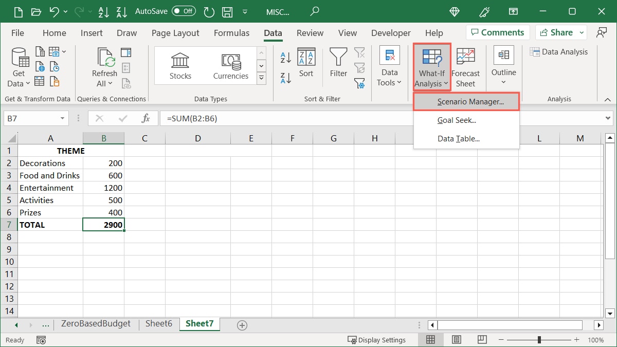
- To add these details to the Scenario Manager, go to the “Data” tab and “Forecast” section of the ribbon. Open the “What-If Analysis” drop-down menu, and choose “Scenario Manager.”
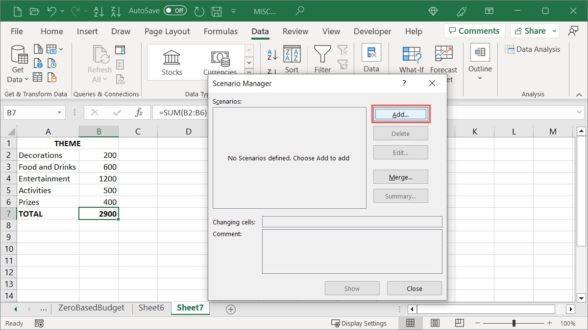
- Click “Add.”
- Give your scenario a name (we are using “Beach Theme”), and enter the cells you’ll adjust in the “Changing cells” field. Alternatively, drag your cursor through the cells in your sheet to populate that field. Optionally, enter a comment other than the default, and click “OK.”
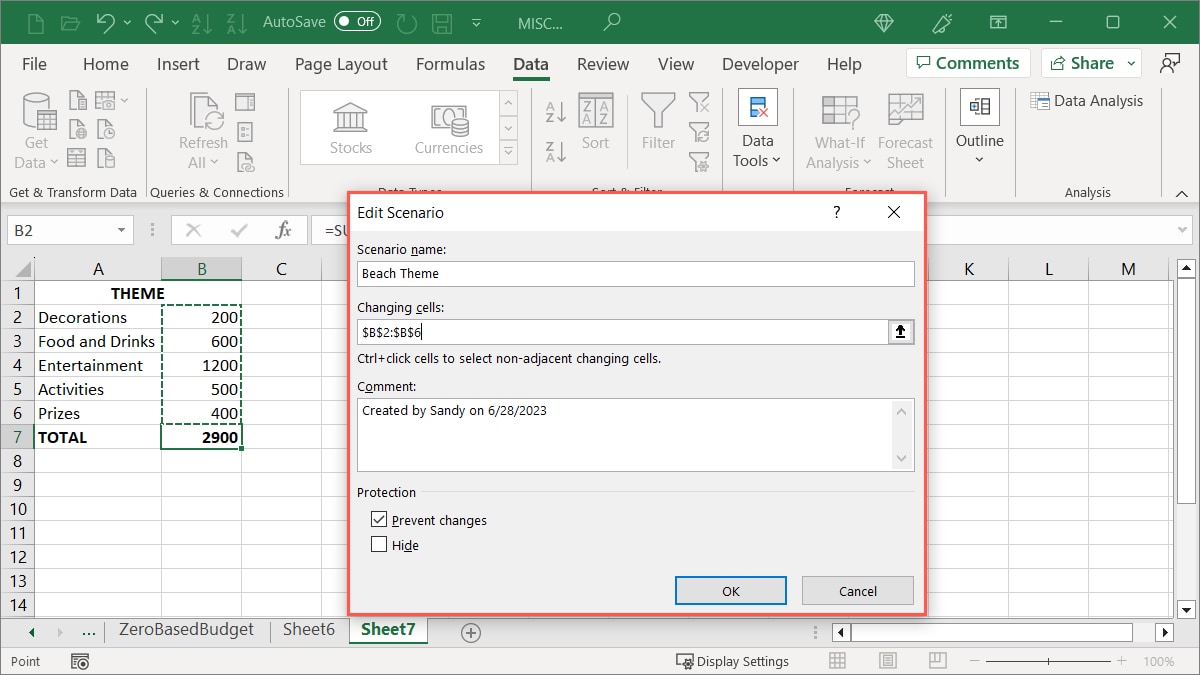
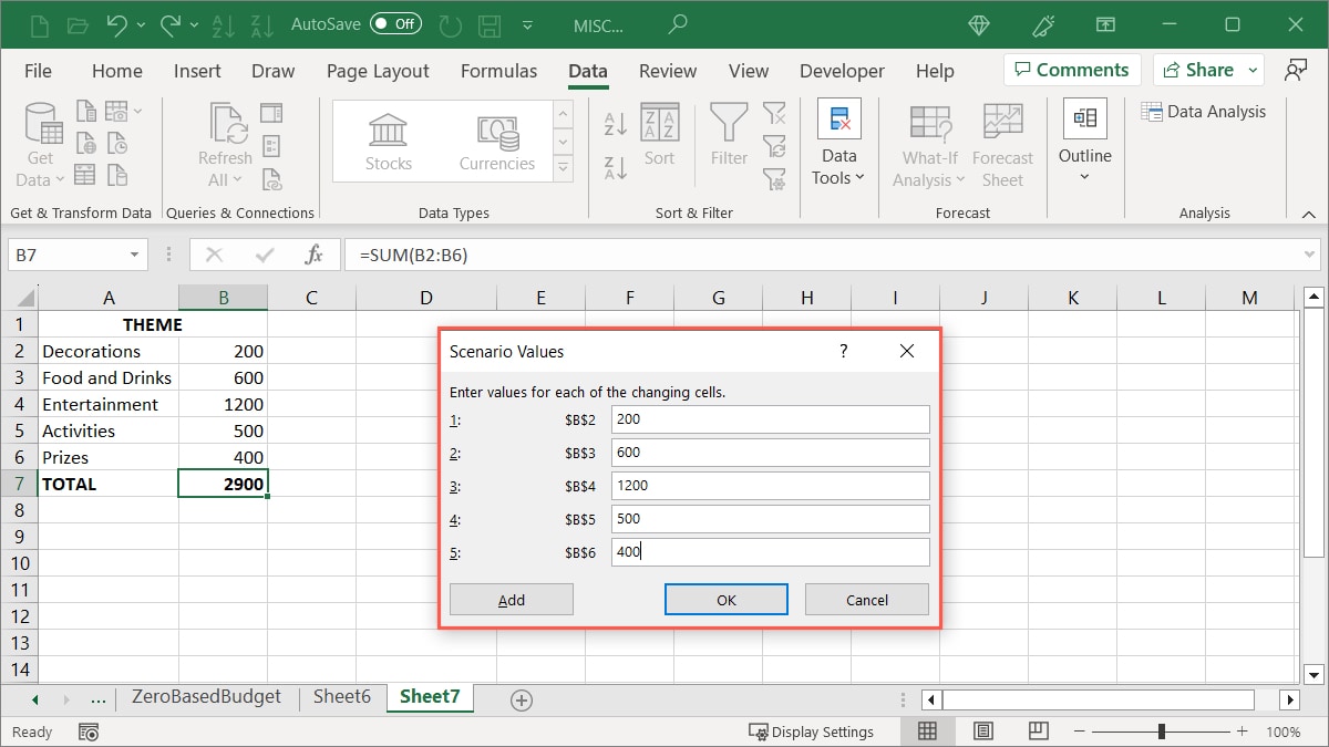
- The values in the “Changing cells” field should match those on your sheet, but you can adjust them here. Click “OK” to continue.
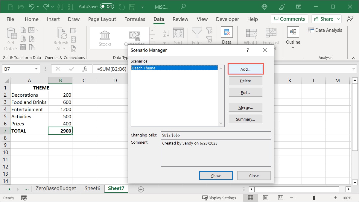
- Now that you’ve added the first scenario, you’ll see it listed in the Scenario Manager. Select “Add” to set up your next scenario.
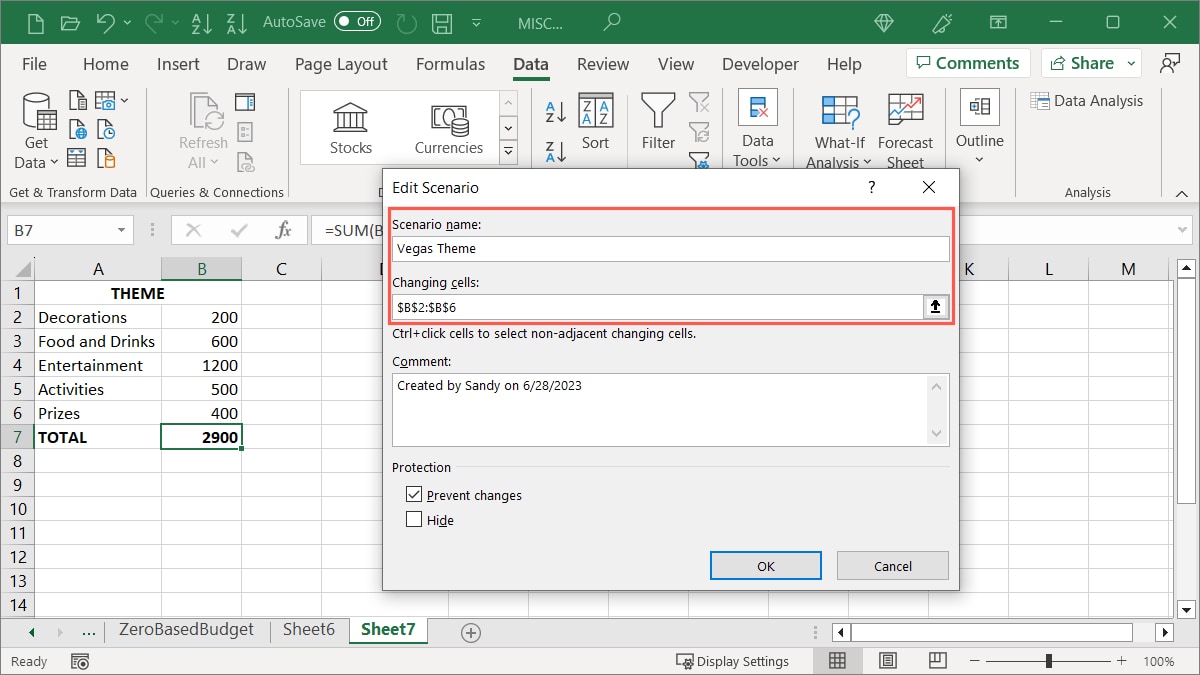
- Enter the details for the second scenario as you did for the first. Include the name, changing cells, and optional comment, then click “OK.” In our example, we are entering “Vegas Theme” and the same cell range, B2 through B6, to easily see an in-place comparison.
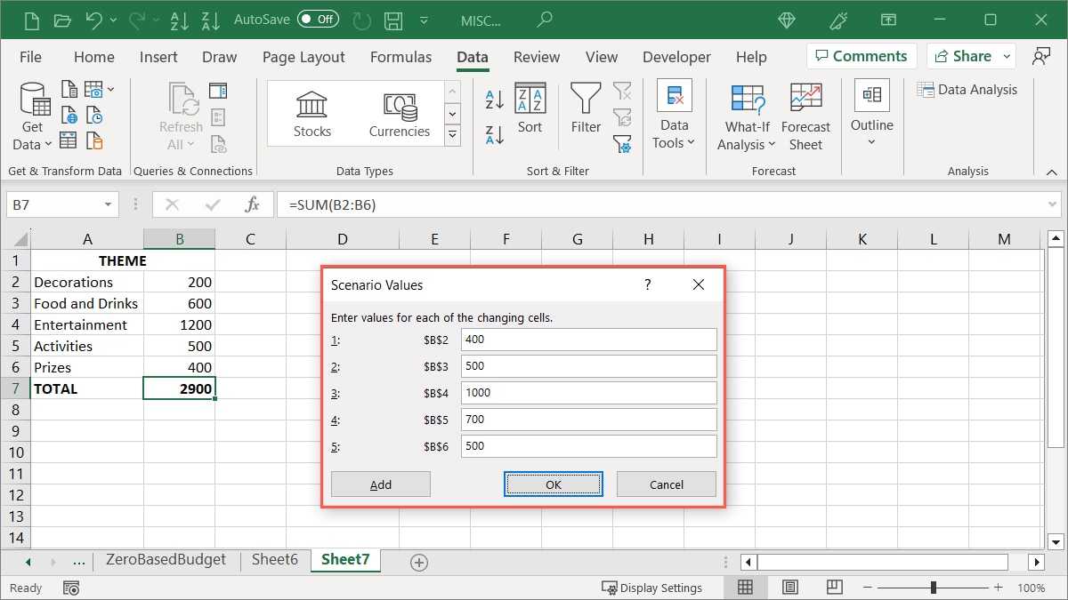
- Enter the values for your second scenario in the Scenario Values window. If you’re using the same cells as the first one, you’ll see those populated. Enter the ones you wish to use, and click “OK.”
- Choose the scenario you want to view from the list in the Scenario Manager window, and click “Show.”
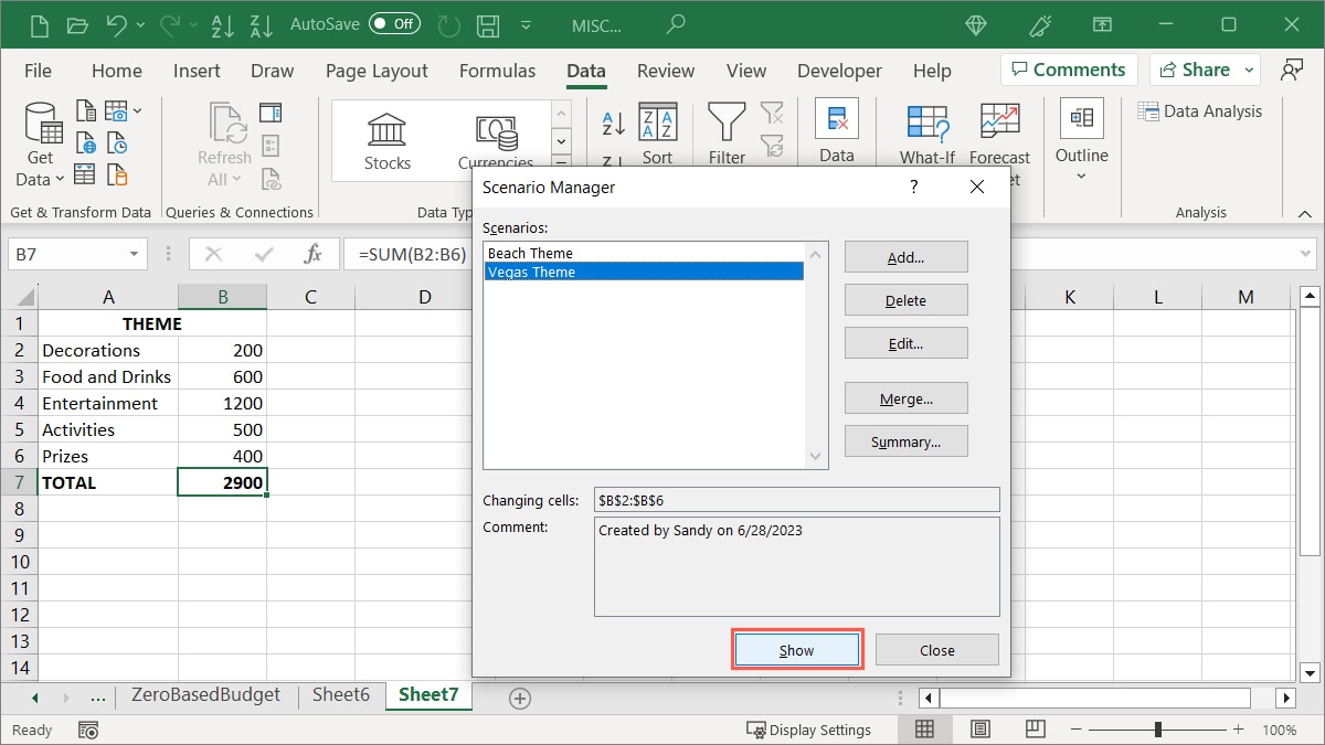
- The values in your sheet will update to display the selected scenario.
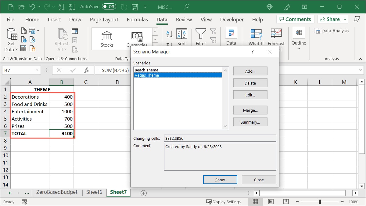
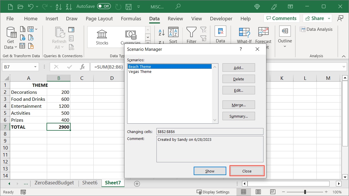
- Continue to add and show additional scenarios to view the updated values in your sheet. Once you find the one you want to keep in your sheet, select “Close” to exit the Scenario Manager.
FYI: do you know you can easily create a mind map in Microsoft Excel?
View the Scenario Summary
View the Scenario Summary to see all of your scenarios at once to perform a side-by-side comparison.
- Return to “Data -> What-If Analysis -> Scenario Manager,” then click “Summary.”
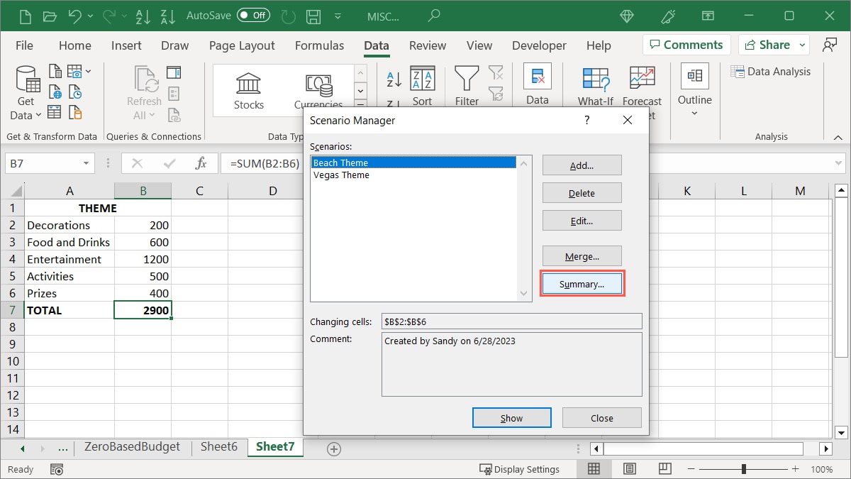
- Choose the report type you want to view: either “Scenario summary” or “Scenario PivotTable report.” Optionally, if you want to display your result, enter the cell that contains it, and click “OK.”
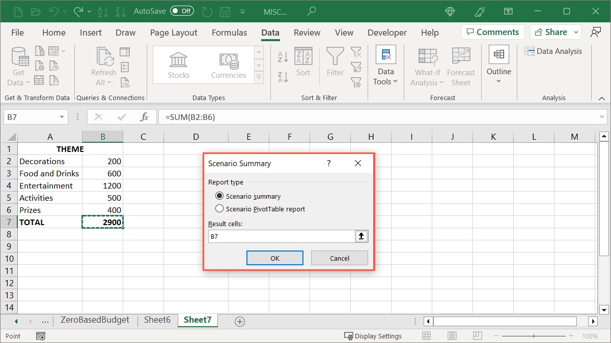
In our example, we are selecting “Scenario Summary,” which places the report in a new sheet tab. You’ll also notice that the report can optionally include cell grouping to hide certain portions of the report.
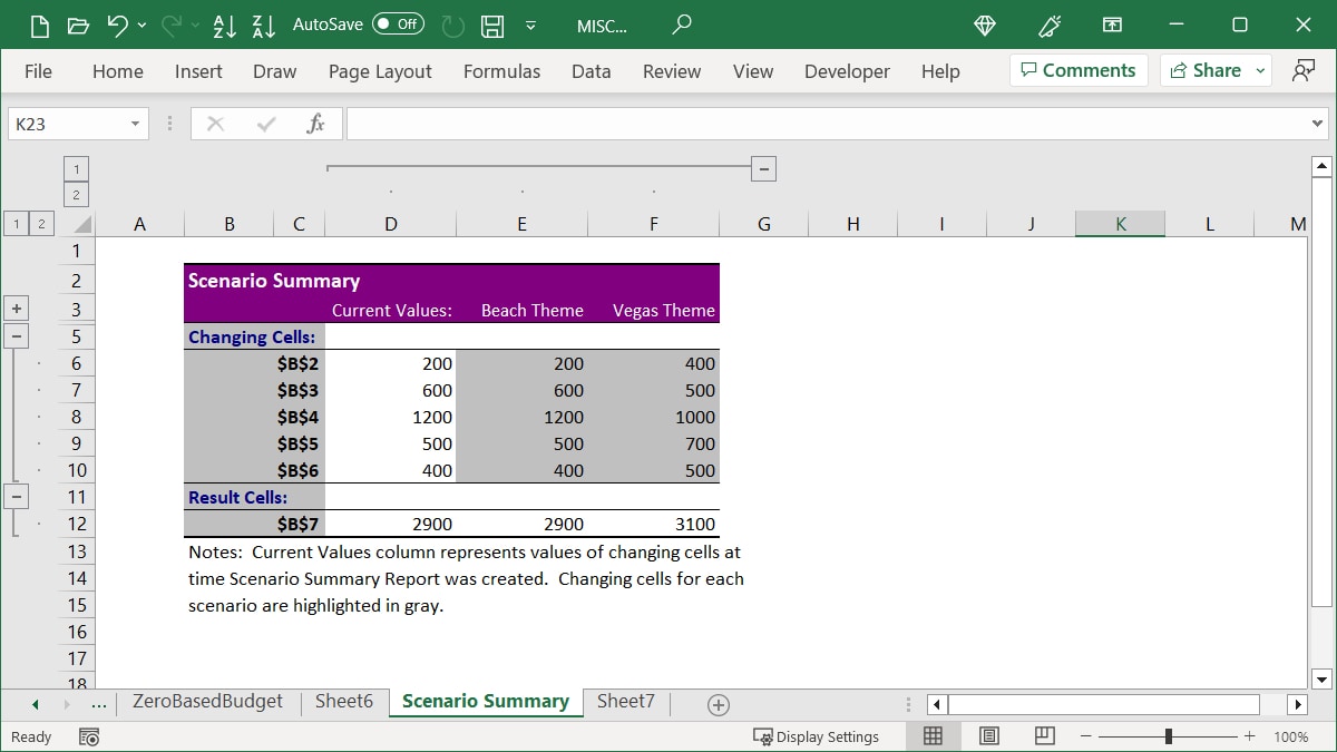
Note that if you adjust the details in the Scenario Manager, the report does not update automatically, so you must generate a new report.
Tip: find out how Excel pivot tables can improve your productivity.
Goal Seek
The Goal Seek tool works somewhat oppositely of the Scenario Manager. With this tool, you have a known outcome and enter different variables to see how you can arrive at that outcome.
For instance, maybe you sell products and have a yearly profit goal. You want to know how many units you need to sell or at what price to reach your goal. Goal Seek is the ideal tool to find answers.
With Goal Seek, only one variable or input value can be used. Use this for those scenarios where you have the remaining values upfront.
How to Use Goal Seek
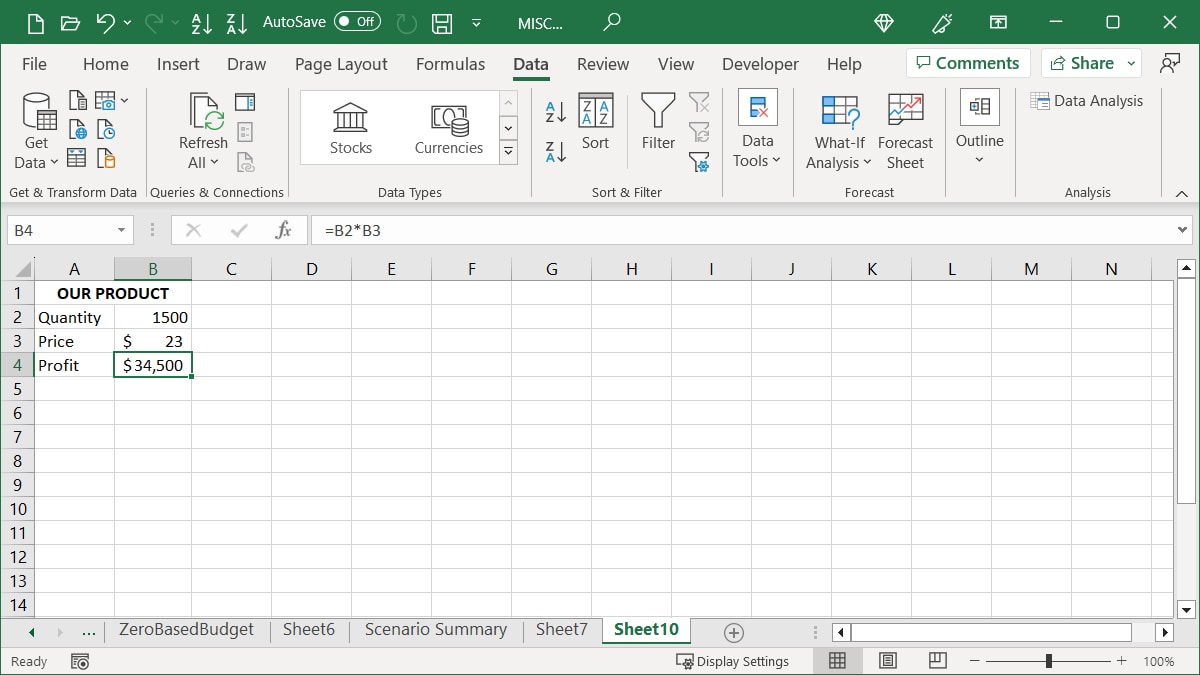
In an example of the Goal Seek tool, we have 1,500 products to sell and want to make a profit of $52,000. We are using Goal Seek to determine at what price we should sell our product to reach that goal.
- Start by entering the values and formulas in your sheet, per your scenario. Using our example, we are entering the current quantity in cell B2, estimated price in cell B3, and a formula for the profit in cell B4, which is
=B2*B3.
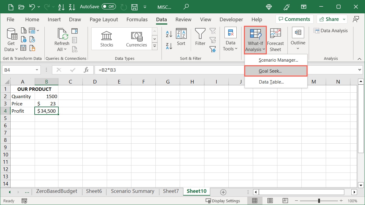
- Go to the “Data” tab, open the “What-If Analysis” drop-down menu, and choose “Goal Seek.”
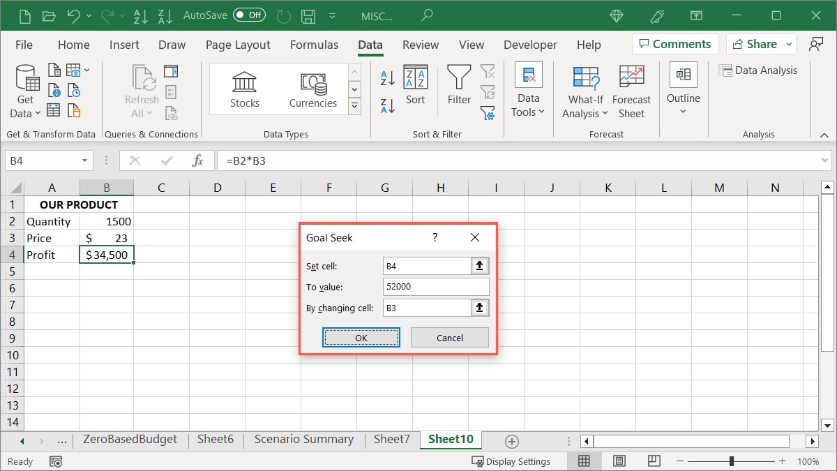
- Enter the following values, then click “OK”:
- Set cell: the cell reference (containing the formula) for the value you want to change to reach the desired result. In our example, this is cell B4.
- To value: the value of your desired result. For us, this is 52000.
- By changing cell: the cell reference you want to change to reach the result. We are using cell B3, as we want to change the price.
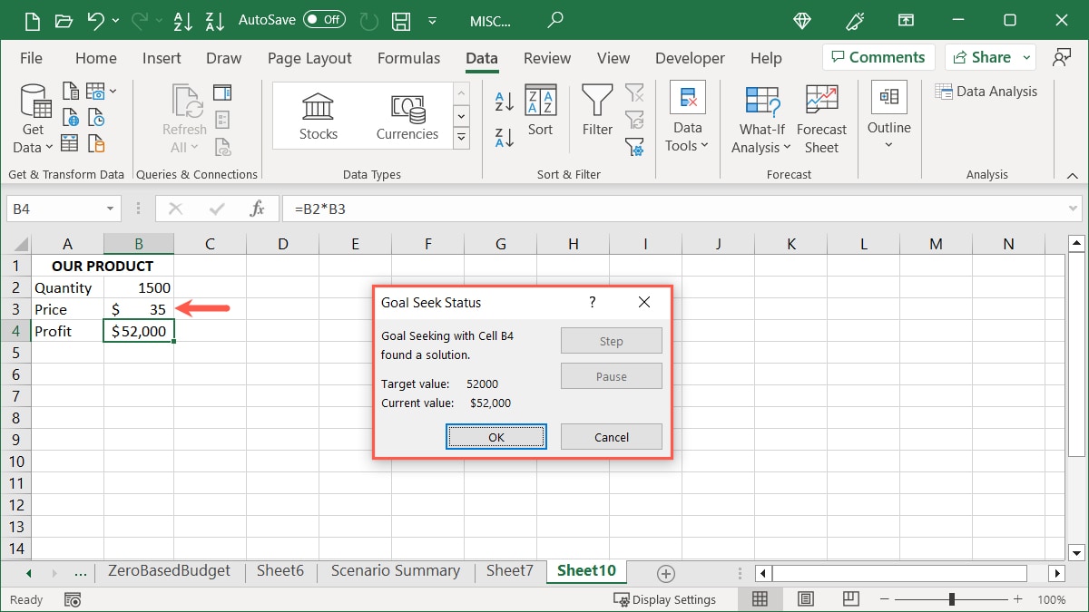
- Click “OK” to see the “Goal Seek Status” box update to display a solution and your sheet change to contain the adjusted values. In our example, we must sell our product for $35 to reach our $52,000 goal. Select “OK” to retain the new values in your sheet.
Do you know: there are plenty of things you can do in Microsoft Excel, including inserting sparklines and mini chart.
Data Table
Use a Data Table in Excel to view a range of possible numeric situations.
For an ideal example, you may be reviewing loan options. By entering different interest rates, you can see what your monthly payment would be with each one. This helps you determine what rate to shop for or discuss with your lender.
With a Data Table, you can only use up to two variables. If you need more, use the Scenario Manager.
How to Use a Data Table
Follow the steps below to use a Data Table, the third What-If Analysis tool. Do note the data setup.
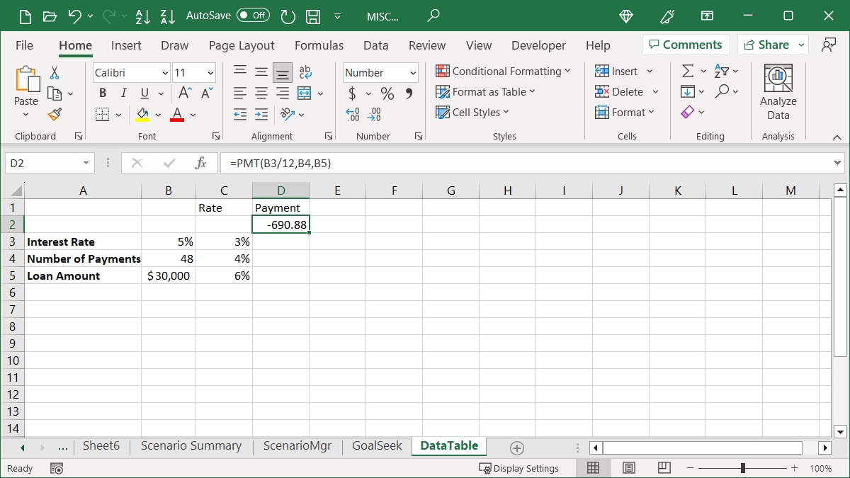
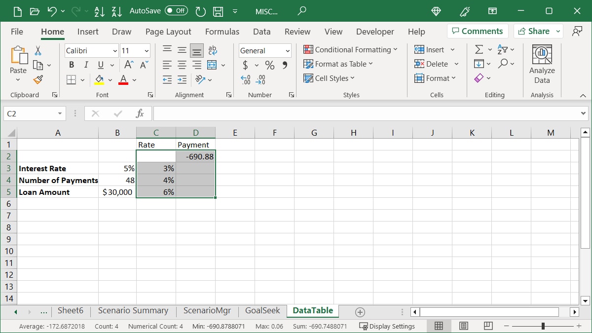
For an example, we are using a Data Table to see how much our loan payments would be with different interest rates via the following data:
- Interest rate, number of payments, and loan amount in cells B3 through B5.
- A Rate column with the interest rates to explore in cells C3 through C5.
- A Payment column with the formula for the current payment in cell D2.
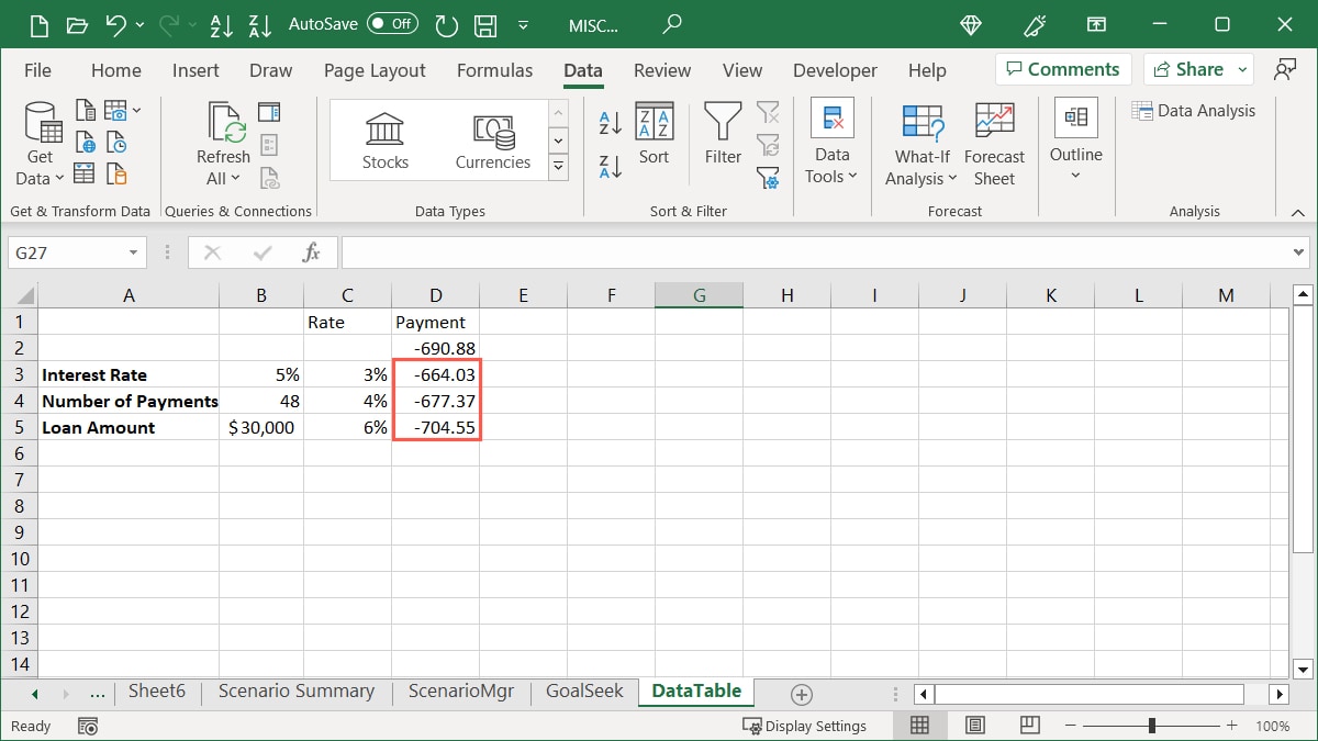
- The result cells below the formula in the Payment column, entered automatically using the Data Table tool. This shows us the payment amounts per interest rate.
When you enter your data and formula in your sheet, keep the following in mind:
- Use a row- or column-oriented layout. It will determine the placement of your formula.
- For a row-oriented layout, place your formula in the cell one column to the left of the initial value and one cell below the row containing the values.
- For a column-oriented layout, place your formula in the cell one row above and one cell to the right of the column containing the values.
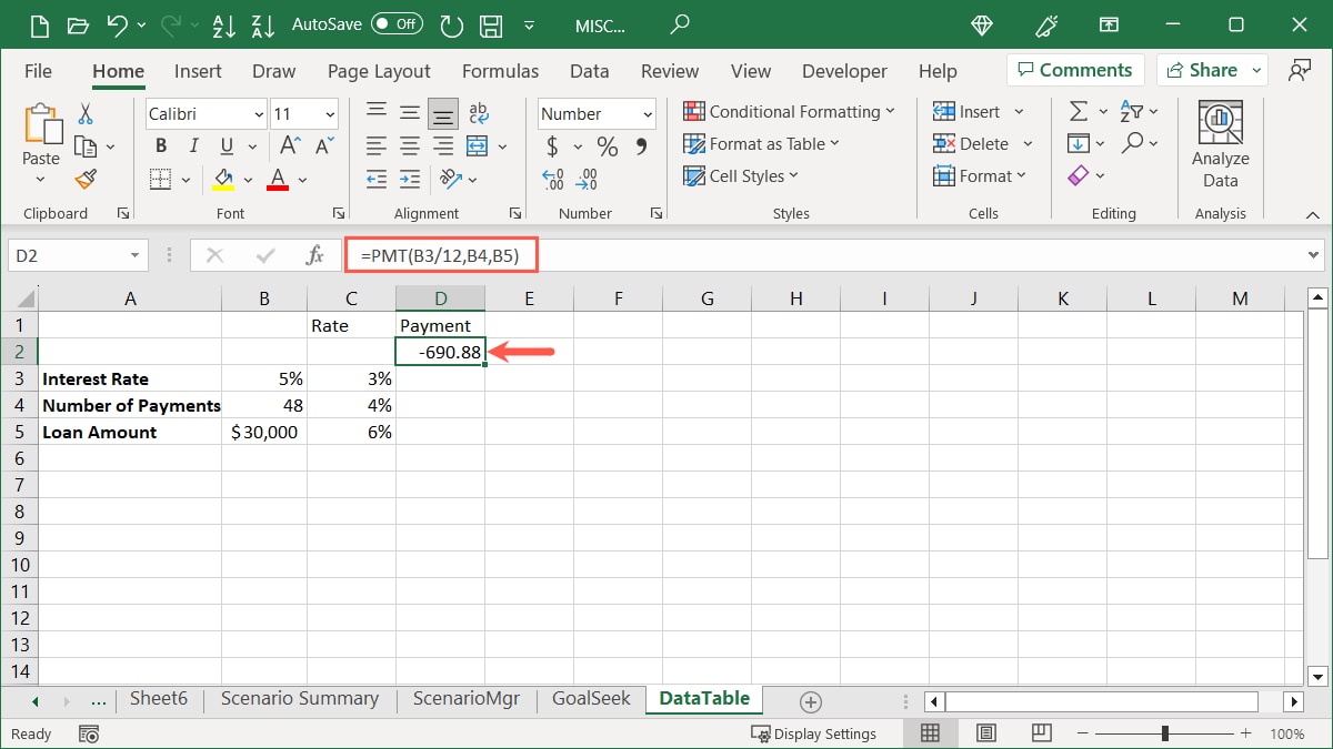
In our example, we’re using a single-variable (the interest rate) in a column-oriented layout. Note the placement of our formula in cell D2 (a row above and one cell to the right of our values).
- Enter your own data and select the cells containing the formula, values, and result cells. In our example, we are selecting cells C2 through D5.
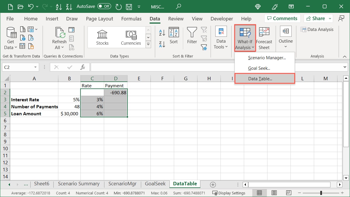
- Go to the “Data” tab, open the “What-If Analysis” drop-down menu, and choose “Data Table.”
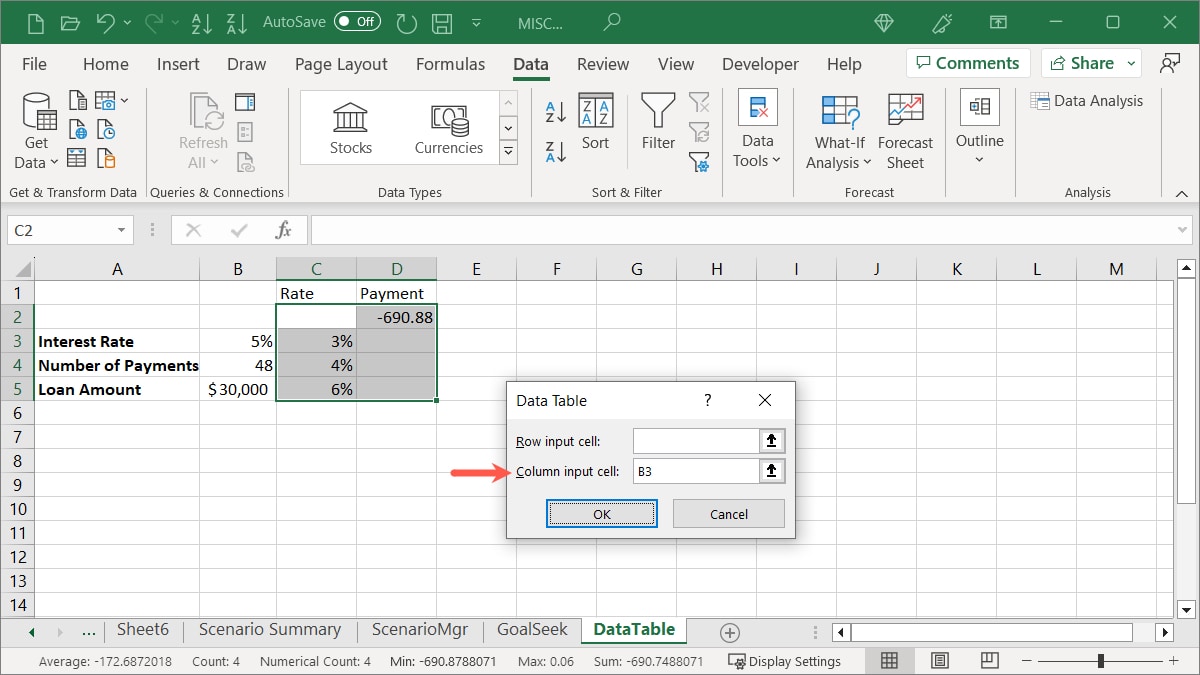
- Enter the cell containing the changing variable for your data into the Data Table box. For a row-oriented layout, use the “Row input cell,” and for a column-oriented layout, use the “Column input cell.” In our example, we are using the latter and entering “B3,” which is the cell containing the interest rate.
- After you click “OK” in the Data Table box, you should see the result cells fill with the data you expect. Our example includes the amount of our payment for each different interest rate.
Note that you can use two variables in your Data Table instead of one, try out the row-oriented layout, or view further details and limitations of this What-If Analysis tool on Microsoft’s Support page for the feature.
Frequently Asked Questions
How do I edit an existing Scenario in Excel?
You can change the name and values for a scenario using the Scenario Manager. Open the tool by selecting “Data -> What-If Analysis -> Scenario Manager.” Pick the scenario from the list, and click “Edit” on the right. Make your changes, and choose “OK” to save them.
If you created a Scenario Summary report initially, you’ll need to regenerate the report to see the updated details.
Can I stop Excel from recalculating a Data Table?
If your workbook contains a Data Table, Excel automatically recalculates that Data Table, even if there are no changes. However, you can turn this option off if you would like.
Go to the “Formula” tab, open the “Calculation Options” drop-down menu in the Calculation group, and select “Automatic Except for Data Tables.”
To recalculate your Data Table manually, select the formula(s) and press F9.
What other analysis tools does Excel offer?
Excel provides many different types of data analysis tools, depending on what you need. To name a few, you can use conditional formatting to highlight specific data, Quick Analysis for formatting, charts, and tables, and Power Query for robust data analysis.
You can also use basic Excel features, like filters, for narrowing down your data, slicers for filtering tables and charts, and the Analyze Data tool for getting answers to questions about your data.
For additional assistance on these features and more, head to the “Help” tab in Excel on Windows, or use the “Tell me” menu option in Excel on Mac.
Image credit: Pixabay. All screenshots by Sandy Writtenhouse.
Our latest tutorials delivered straight to your inbox